Determination of the Force Constant
of a Helical Spring by the Oscillation Method
Plot the T²–m graph to determine the force constant and effective mass of a given helical spring.
Objective
Section 01Aim
To determine the force constant and effective mass of a given helical spring by plotting a T2–m graph using the oscillation method.
Learning objectives
- Understand the oscillatory motion of a spring-mass system.
- Measure the time period for different suspended masses.
- Determine the force constant from the slope of the T2–m graph.
- Determine the effective mass from the intercept of the graph.
Theory
Section 02Force constant
The force constant (or spring constant) of a spring is the restoring force produced per unit extension.
When a mass is suspended from a spring and displaced slightly from its equilibrium position, it performs simple harmonic motion.
Effective mass of the spring
If the spring, hanger and attached system have an effective mass m0, the time period becomes:
Squaring this equation gives:
Graphical determination
Plot T2 on the y-axis and m on the x-axis. If the slope is a and the y-intercept is b, then:
The SI unit of K is N m−1 and the SI unit of m0 is kg.
Precautions
- Use a small amplitude and release the load gently.
- Allow the pointer to come to rest before starting an observation.
- Measure the time for several oscillations to reduce timing error.
- Keep the spring within its elastic limit.
Apparatus Required
Section 03Apparatus
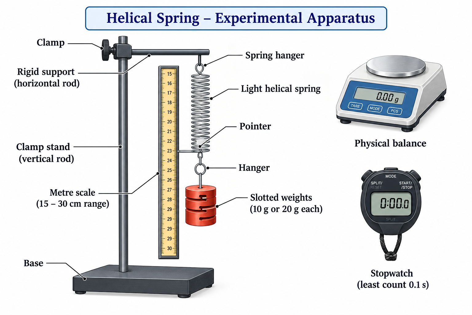
- Light helical spring with a pointer and hanger.
- Rigid support and clamp stand.
- Hanger and slotted weights of 10 g or 20 g.
- Physical balance.
- Metre scale (15–30 cm).
- Stopwatch with least count 0.1 s.
Procedure
Section 04Real experiment
- Suspend the spring from a rigid support and attach the pointer and hanger to its lower end.
- Place a vertical metre scale beside the spring without touching the pointer.
- Determine the least count of the scale and stopwatch.
- Hang a known mass m gently and wait until the pointer comes to rest at the equilibrium position.
- Pull the load slightly downward and release it gently. Start the stopwatch as the pointer crosses the mean position in a fixed direction.
- Record the time t for n oscillations. Repeat at least three times and calculate the mean time.
- Calculate the time period using T = t/n. Repeat for different masses.
- Calculate T2 for each mass and plot the T2–m graph. Determine K and m0 from its slope and intercept.
Virtual experiment
- Open the Simulation section and pause the simulation.
- Set the load mass and take the pointer position as the mean position.
- Play the simulation. Start the stopwatch as the pointer crosses the mean position in a fixed direction.
- Count n oscillations and stop the stopwatch immediately after n complete oscillations.
- Repeat the timing at least three times and calculate the mean time period using T = t/n.
- Repeat the measurements for different masses and record the readings in the observation table.
- Use the simulation plots to analyse the readings: Time Period (T) vs Mass of Load (m), T2 vs Mass of Load (m), and Mean Position of Pointer (y) vs Mass of Load (m).
- Use the data and fitted plots to calculate the Force constant, K, and the Effective mass, m0 in the Result and Analysis section.
- Enter the calculated values in the appropriate input boxes, then click Export PDF to export the completed experiment report as a PDF.
Simulation
Section InteractiveObservation Table
Section 06Spring oscillation observations
Result and Analysis
Section 07Calculation
For two readings:
From the T2–m graph, if slope = m′ and intercept = c′:
Record your calculation
Assessment
Section CheckHelical Spring Experiment – MCQs
Select the most appropriate answer.